Searching For Historic Noise
A Study of a Sound Recording Made on the Day of the
Assassination of President John F. Kennedy
Robert Berkovitz, Sensimetrics Corporation
On November 22,1963, the day President John F. Kennedy was assassinated, the Dallas Police Department (DPD), like the police in many other cities then and now, recorded police radio communications automatically. The police and others realized only later that the recordings routinely made that day might be useful in investigations of the assassination. Although witnesses had claimed to have heard a second gunman shooting at the president, the Warren Commission, appointed by President Johnson to investigate the assassination, had found no evidence of a second assassin. When it appeared that one of the police recordings might contain the sounds of the assassination gunfire, a committee of the U. S. Congress, the House Select Committee on Assassinations (HSC), asked the acoustical consulting firm Bolt Beranek & Newman (BBN) to study the recordings to determine what could be learned from them about the assassination. Mark R. Weiss and Ernest Aschkenasy (WA) of the Computer Science Department at Queens College (C.U.N.Y.) in New York, were subsequently also asked to study the recordings.
The three reports cited in the text as BBN, WA and NAS are listed at the end of this report.
Each police motorcycle radio transmitter had a push-button on its microphone that had to be pressed when the user wanted to talk. Pressing the button switched on the transmitter; when the button was released, it would spring out and the transmitter would be shut off.
A few minutes before the assassination, the push-button on one motorcycle transmitter was not released. For about five minutes, until the problem was corrected, the transmitter on that motorcycle apparently broadcast continuously. This accidental five-minute transmission, which continued through the time of the assassination, was recorded automatically at the police communication center.
The recording equipment used at Dallas police headquarters was primitive even by 1963 standards. Although magnetic tape recording was already in widespread use elsewhere, the two Dallas recorders were mechanical and made recordings using the same principle as the phonograph record invented a hundred years earlier. Two channels were used for police radio transmissions and two devices recorded the transmissions. One machine, recording transmissions on radio Channel 1, recorded by scratching a groove in a moving belt of soft, flexible plastic, called a Dictabelt™. To hear the recording, a needle was put in the groove and the belt again set in motion. A second machine, a Gray Audograph™, recorded radio Channel 2. Instead of a plastic belt, the Audograph recorded on a plastic disk almost as thin as a sheet of paper. The Audograph traced its groove from the center of the disk to the outside, the opposite of a phonograph record. Unlike a phonograph record, the Audograph disk did not turn at constant speed, but turned faster at the start of a recording, then slowed as the recording needle moved outward. This made the needle move the same distance each second, even though the spiral track was larger in diameter at the outside of the disk. Both the Dictabelt and Audograph media were made of soft plastic and were therefore delicate, so that scratches and dust particles on their surfaces added click- or pop-like transient impulses during playback.
Investigators reasoned that if the motorcycle had been in the presidential motorcade when it passed through Dealey Plaza, where the assassination took place, the recording would contain the sounds of the three gunshots allegedly fired by Lee Harvey Oswald. If the sounds of more than three shots were found in the recording, that might indicate that a second assassin had fired. If there had been more than one assassin, the assassination might be the result of a conspiracy in which the shooting had been coordinated. If no more than three shots were found, conspiracy theories requiring two assassins would need to be abandoned.
BBN had devised a method of analysis that could be applied to the Channel 1 recording that could locate the sources of gunshots recorded in a reverberant environment. There are a number of buildings and other structures surrounding Dealey Plaza, and the sound of a gun fired in the plaza would be reflected from the buildings. For each possible location of gun and microphone, there would be a unique pattern of echoes following the sound of the shot. By measuring the time intervals between the shot and each of its echoes and relating these measurements to surrounding structures, the locations of the gun and motorcycle could be established.
To apply the method, which had already been used successfully in an earlier case, BBN investigators had rifles fired from the window in Dallas where Oswald is said to have hidden, and from behind a fence on a grassy knoll, where some witnesses said they had heard a shot. Recording microphones were placed on the street several meters apart along the path taken by the presidential motorcade.
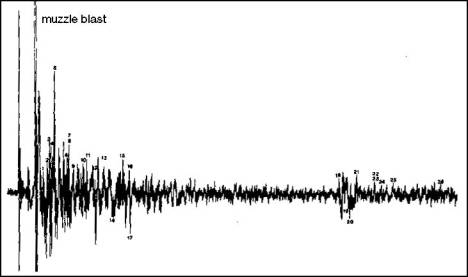
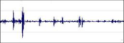
Figure 1 Waveform of a gunshot and its echoes recorded in Dealey Plaza by BBN investigators in 1978 (illustration adapted from the WA report), filtered to simulate the effects of the police radio equipment. The waveform consists mainly of a series of spikes or impulses. The image has been cropped at the top and bottom; in the original illustration, the muzzle blast is larger than shown here. The numbers refer to echoes from specific buildings.
The waveform of each recording of a test shot showed a shock wave and muzzle blast followed by a series of echoes from the buildings surrounding the plaza. Each test recording was measured to find the time between these events. The motorcycle recording made on the day of the assassination was then searched to find groups of shots and echoes that matched the measurements of test shot recordings.
Searching through the recordings, then fifteen years old and quite fragile, investigators found a number of groups of impulses with timings resembling echoes in the test recordings. Since the police recording contained many impulsive sounds undoubtedly caused by static, scratches or defects in the delicate plastic Dictabelt, a standard statistical correlation test was used to estimate the likelihood that the matches were genuine and not accidental.
Four of the patterns matched the tests better than others, with binary correlations greater than 0.6, the minimum set by the investigators for an echo pattern to be examined further. Comparing these groups of impulses to the test recordings, BBN found that three groups matched echo patterns of test shots fired from the Texas Schoolbook Depository and recorded along the path of the presidential limousine. These were judged to probably correspond to the shots allegedly fired by Lee Harvey Oswald. An additional group of impulses, between the second and third shots attributed to Oswald, matched the echoes of a test shot fired from the “grassy knoll.” The BBN investigators assigned a probability of 50% to the presence of a shot fired from the grassy knoll at this place in the recording.
The BBN report to the subcommittee contains pictures of the waveforms of each of the four impulse groups said to be the assassination gunfire and its echoes. These are shown in figures 2 through 5. For comparison, we have included images of the same places in the recording used in our investigation. In each pair, the upper image is reproduced from the BBN report to the subcommittee, and the lower image is one made with our computer, aligned with the BBN image above it. The images from the report differ by being energy plots, while ours are waveform plots. Although the images are different, the times between impulses on the waveforms appear to be nearly identical.
BBN reports that four shots occur at 137.7, 139.27, 145.15, and 145.61 seconds from the start of their timeline. The report notes, however, that these times may not be correct.
Frequency analysis of the power hum on the tape recording also indicated that the recorder had been about 5% slow. Since the hum could have been added when the tape was recorded from the dictabelt, this is not a reliable indication of the original recording speed.
If the recorder ran too slowly, playback at the correct speed would make time appear to pass too quickly reducing the time between echoes. This is the “Munchkin effect,” the method used to create voices for creatures in the film The Wizard of Oz, and many other films and music recordings. To hear the original sound, the recording must be played back at the slower speed used during recording.
In the text of the BBN report, the time given for the first shot is 137.7 seconds. However, this is the time of the third echo (the fourth numbered peak), not the gunshot, in Figure 2, where the first shot is shown to occur 0.2 second earlier than the time given in the text. There is an apparent dislocation between the patterns of shots 1 and 2 (Figures 2 and 3). The starting times of the patterns, that is, the times of the alleged gunshots, may have been chosen to obtain the highest correlation. However, the pattern in Figure 3, which begins with a cluster of impulses, more closely resembles the pattern of Figure 2 when shifted to the right, so that shot 1 happens a fraction of a second later (also see Figure 21).
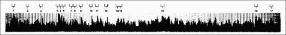
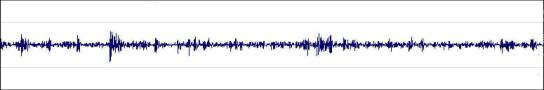
Figure 2 Shot 1 Time, 137.7 seconds, scale 1.12 seconds.
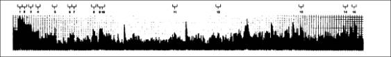
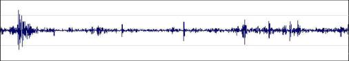
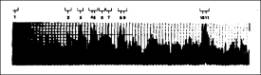
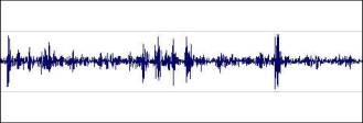
Figure 4 Shot 3 Time 145.15 seconds, scale (lower figure) 0.68 second.
One of the first steps taken by BBN was to print out the waveform of the five-minutes recording on a long roll of paper. The waveform was then searched to find groups of impulses that matched sounds of the test shots fired in Dallas. The BBN report describes the procedure.
The recorded outputs from both filters for the full 5 minutes were compared, examined, and plotted on a scale where 5 in. equals 1/10 sec. …
First, we made a high-resolution graphical plot of the waveform of this signal, at a scale of 5 in. per 1/10 sec, for detailed visual examination. The plot of the entire interval comprises a roll of paper 12 in. wide by 234 ft long. … The region from 144.8 to 147.2 sec, which does not appear in Fig. 4, also contains a large number of impulses of similar character. Because this region is about twice as long as the preceding ones, it was identified as possibly representing two separate impulse patterns, and, therefore, as potentially containing the sounds of two shots.
At the scale described in the text, one second of the recorded waveform would require 50 inches (1.27 m) to plot. The BBN report states that the roll of paper containing the plotted interval was 234 feet (71.32 m) long. If the scale of 50 inches per second is correct, the waveform plot would contain 56 seconds of data, rather than five minutes. On the other hand, if the data were plotted in five parallel lines across the paper, the stated length of the plot would be correct, although the individual waveforms would be only two inches high, possibly making accurate visual examination difficult. In later work by the WA group, analysis of periods as brief as 50 milliseconds is done. On the same scale, a plot of this duration would be only 2.5 inches long.
The description of the recording in the BBN report continues, here describing a spectrogram:
… Just after 144 sec, a single loud click occurs, followed by a region of very faint speech (faint diagonal and horizontal smudges that change rapidly), clicks (thin vertical lines), and keying heterodynes (steady horizontal bars).
This region, which contains the impulses identified as shot 3, was later subjected to further investigation by WA. WA found the best statistical validation of a shot from the grassy knoll would be obtained if the start of the shot was relocated to an impulse about one-quarter second earlier than the impulse chosen as the muzzle blast by BBN. The text of the BBN report explains that the time of shot 3 was changed to agree with WA, although the picture of shot 3 (Figure 4) does not show this correction.
Because of the importance of the finding that there may have been a fourth shot, the WA investigation was devoted to a study of this group of impulses, applying a more stringent test of matching than that used earlier.
WA reported that four shots had been fired, the third shot originating from the fence at the grassy knoll. They found the probability of the data being a coincidence 5%, and described this as a 20-to-1 probability that there had been a grassy knoll shot. This figure and other details of the WA study were included in the BBN report. The subcommittee reported that objective evidence of a second assassin had been found.
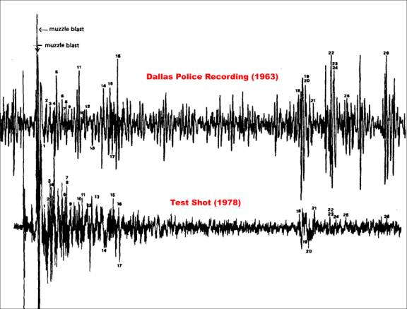
Figure 6 Impulses found in the Dallas Police recording of November 22, 1963 (upper part of figure), and echoes for a test shot from the grassy knoll (lower part, taken from Figure 6 in the WA report). The figures appear separately in the WA report, and have been combined here.
The upper part of Figure 6 contains a plot of the waveform of the recording said to be shot 3, recorded in 1963, as it appears in the WA report to the congressional subcommittee. The lower part of Figure 6, from the same report, is the recording of a test shot fired from the grassy knoll, after filtering to simulate the effect of the microphone on the police radio. Each of the small numbers near the waveform indicates an echo found in both waveforms. We have adjusted the horizontal scale of the two illustrations to make visual comparison of the plots easier.
Figure 6 indicates why statistical methods were needed to estimate the likelihood that a match could be false, that is, the probability that a burst of noise of indeterminate origin was mistaken for a recording of a gunshot. The origins of the individual impulses in the 1963 recording were unknown at the start of the analysis. The noises could have been the sounds of gunfire and their echoes, but they might also have been caused by static, dirt in the groove of the recording, or scratches, bubbles or other surface defects in the plastic Dictabelt.
In the WA investigation, the echo times used for reference were calculated. Here is a description from the WA report.
The only practical way to obtain the needed echo sequence was to predict them analytically. Using fundamental principles of acoustics, it was possible to compute the time it would take for the sound of a muzzle blast to travel from a gun at any assumed point on the grassy knoll to a microphone at any assumed point on Elm Street. Knowing where the echo-producing objects were in Dealey Plaza, it was also possible to compute the time it would take for echoes of the muzzle blast to travel from the gun to the microphone. Subtracting the muzzle-blast travel time from the echo travel times yielded the required sequence of echo-delay times.
…Before the echo travel times could be calculated, it was necessary to determine three things: (1) Which objects in Dealey Plaza would produce echoes in the region of interest on Elm Street for a gun fired from the vicinity of the grassy knoll; (2) how far these objects were from the locations of the gun and of the microphone; and (3) what was the speed of sound under the conditions for which the echo travel times were to be predicted. When the required information had been obtained, it was used first to determine the accuracy of the echo procedure. Then it was used to predict echoes for comparison with the impulses in the DPD recording. …
These waveforms…were obtained by playing back the recording of the sounds that were picked up by the microphone, modifying the reproduced signal so as to approximate the effect that a microphone of the type used by the DPD in 1963 would have had on the signal, and then graphing the resulting signal [the lower portion of Figure 6]. … The first waveform appearing in the graph, the large peak at the left-hand side, corresponds to the supersonic shockwave of the rifle bullet. The second large peak is the waveform of the muzzle blast. Following it, with generally diminishing heights, are the waveforms of the echoes of the muzzle blast. The delay time of each echo was determined by direct measurement of the distance from the leading edge of the muzzle blast waveform to that of the echo.
The WA calculations produced a table (Figure 7), in which the predicted echo times (“Echo delay time”) are compared to those found by measuring the times of actual impulses found in the 1963 recording (“Impulse delay time”). The levels of the impulses were disregarded. The match of the two sets of impulses was close, as can be seen in the small deviations, and was consistent with the presence of an assassin on the “grassy knoll.” The amplitudes of the impulses and echoes were judged to be inapplicable, presumably due to non-linear effects of the electronic circuitry.
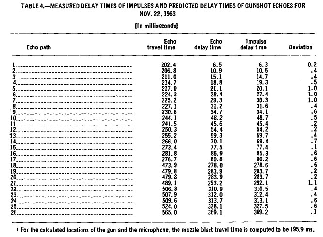
Figure 7. Reproduction of Table 4 from the WA report showing predicted “Echo delay time” and “Impulse delay time,” the time of the corresponding impulse found in the 1963 police recording.
A few years later, at the request of the Department of Justice, a special committee was appointed by the National Academy of Sciences (NAS) to assess the methods used in the earlier investigations and to make recommendations for further study of the recordings. The committee, named the Special Committee on Ballistic Acoustics, concluded that the reports to the congressional committee had arrived at conclusions that were incorrect because the methods used were faulty, important evidence had been overlooked, and inappropriate subjective judgment had been applied. The NAS report questioned the specific statistical methods used to test the validity of the results. The NAS published detailed evidence indicating that the sounds cited as those of the assassination had been recorded after the assassination. The latter evidence, the committee pointed out, invalidated any conclusions drawn from the similarity of the noises on the Dictabelt to the sounds of gunshots.
We examined several of the available copies of the Channel 1 Dictabelt recording using laboratory instruments and computers. We considered the results of previous studies of this recording and weighed both critical and approving comments about the BBN and WA reports. We created a computer program, IMPULSES, to assist in analyzing the data, especially to reduce manual and visual measurement work, with the aim of obtaining more accurate results.
Our work can be summarized as follows.
1. We digitized recordings of Channels 1 and 2 and examined their waveforms on a computer screen. We compared the noise identified as the grassy knoll gunshot and its echoes to the echoes calculated and listed in the WA report. We applied the statistical tests used by BBN and WA.
2. We studied a voice message heard on the Channel 1 recording during the series of sounds identified as shots 3 and 4, to learn whether the voice and the shot-like sounds were recorded at the same time.
3. We compared different copies of the Channel 1 recording, including a copy of the version used by BBN and WA, to copies made earlier and later by the Dallas Police Department and the F.B.I..
4. Much of the five minutes of the Channel 1 recording consists of continuous noise. We sampled and analyzed the noise for clues to the location of the transmitting microphone.
5. Specific voice messages appearing on Channels 1 and 2 have been offered as time references, indicating that the sounds identified as gunshots were recorded at the time of the assassination, not later. We analyzed the voice message recordings to test this possibility.
We began by disregarding arguments that the data in question was recorded after the assassination. In locating the recorded muzzle blast of a gunshot, we accepted as a potential gunshot the set of impulses imbedded in noise and found to be separated by time intervals corresponding to those in the set of predicted echoes.
The task confronting the original investigators required two difficult problems to be solved. First, as much irrelevant noise as possible had to be removed from the signal, if it could be identified. Second, the accuracy of the match between recorded impulses and predicted echoes had to be evaluated statistically, as the nature of the recording process and the conditions of recording made a perfect match unlikely. The investigators therefore offered their conclusions in the form of probabilities, not certainties.
By any standard, the quality of the police recording is poor. In addition, the transformations of the sound signal during transmission and recording, especially non-linear effects, are uncertain. As a result, the expected amplitudes of the echoes, potentially important comparative data, are unknown.
The WA report describes two tests. Visual examination of figures in the WA report indicates that in the first test, the contents of approximately 370 milliseconds of the DPD recording of the DPD recording were examined. According to the report, 13 echoes, including the muzzle blast, would have been loud enough to appear above the threshold they set to reduce interference by low-level noise. They counted a total of 15 impulses with peaks that were above the threshold, of which 11 were not more than a millisecond earlier or later than the predicted time of an echo. The report does not state which impulses in the recording or which of the predicted echoes, exceeded the threshold, or which matched within the ±1 millisecond tolerance.
The investigators explain that electronic circuits in the communication system would have distorted the amplitudes of the recorded impulses, especially during approximately the first 1/20th second after the muzzle blast. Presumably, this is the reason for the absence of data regarding the correlation of impulse amplitudes and predicted echo amplitudes. Especially at the end of the series of echoes, there appears to be a substantial negative correlation of the amplitudes of impulses and predicted echoes.
To estimate the likelihood that a group of impulses is a recording of a gunshot and its echoes, and not an accidental match to noise in the recording, the correlation between the two patterns is calculated. In the report of the original investigators, three quantities were used to make this calculation: (1) the number of echoes that would have occurred during the time period examined, (2) the number of impulses that matched such echoes, and (3) the total number of impulses in the period.
In effect, two recordings are being compared. One is the relatively crude recording made on a Dictabelt in 1963 (or a tape copy made from it), and the other a high-quality recording of a test shot fired in 1978. Ideally, the data in the new recording, made with modern, highly accurate apparatus, would be subjected to the same transformations as those imposed by the relatively crude equipment used to make the 1963 recording before the sounds in both were compared.
The loudness of echoes and impulses did influence the results of the procedure used by the investigators indirectly. When a threshold level is chosen to suppress low-level noise, the number of possible matches is limited to the number of predicted echoes that exceed the threshold. Since the threshold is an amplitude level, it must correspond to the same acoustic level in the echo pattern calculated in 1978 and in the 1963 recording.
Here are some observations by the original investigators.
4.5 Amplitude of Impulses
Another characteristic of the waveforms that would have been affected by the circuitry of the radio transmitter if the input signal was as loud as gunfire was their amplitude. The recorded amplitudes of the sounds would be compressed in such a way that strong signals would appear to be weaker than they actually were, and weak signals in the same pattern would, therefore, appear stronger. As can be seen in Fig. 11, this compression is greatest for very loud signals, especially those with high-frequency content. For example, although all the signals were compressed, the amplitude compression of muzzle blast waveforms above 100 dB was in every case less than that of the shock waves that are of higher frequency.
When the peak-to-peak difference in amplitude between two signals was 30 dB, they were recorded as having only a 20-dB difference (muzzle blast) or only a 10-dB difference (shock wave). As the amplitude of the input signal decreased, the difference in peak-to-peak level became more noticeable. This analysis gave us greater insight into the characteristics of the sounds originally recorded on the DPD tape. The signals on that tape also appeared to be compressed in amplitude, indicating that the sounds, as originally picked up at the motorcycle microphone, may have been loud enough to have been caused by gunfire.
The treatment of negative impulses in determining the correlation coefficient is not clear. In the 370-millisecond period examined, the investigators predicted five echoes corresponding to negative-going impulses in the test shot waveform (echoes 1, 14, 17, 19 and 20), the last two at 283.9 milliseconds after the muzzle blast. In Table 4 of the WA report, no polarity or amplitude information is given for the impulses or echoes, but in Figure 7, only three negative impulses are identified as matching echoes, all in the first 90 milliseconds. In the statistical tests, only positive impulses (in the display convention depicted in the reports) appear to have been counted.
The following explanation of the use of a threshold is from the BBN report:
Since impulse patterns that are truly caused by gunfire and mixed with radio noise cannot be expected to correlate perfectly with the test patterns, the detection threshold must be set low enough to ensure that no detections are missed. But the lower the detection threshold is set, the more false alarms that can be expected to occur. The analysis described in Appendix C indicated that random noise on one 1-sec segment of the DPD tape having about 12 impulses per sec will cause fewer than 3.3 false alarms out of 432 echo patterns, provided the detection threshold is 0.6. This rate of false alarms was judged acceptable and was considered necessary to prevent misses.
In addition to examining the waveform of the Dallas recording, the investigators examined the energy of the recorded signal. This had two effects on the data; it eliminated the polarity of the impulses, and since the energy is plotted on a logarithmic scale (in dB), lower-level impulses are made proportionately larger visually. The measurements made by WA were apparently made using waveform plots, according to the testimony given to the subcommittee.
Should negative impulses be tallied and considered in calculating the correlation of the 1963 recording to the test shot recording? From the testimony of Dr. Weiss, it is the peak level of an impulse and its precise timing that are of primary interest. For this reason, negative impulses in one recording that correspond to positive impulses in the other are to be treated in the same way as impulses that have the same polarity in both recordings.
Mr. WEISS - Dr. Barger's wave form here represents
the total power or strength of the signal as we see it. The problem here was
to actually be able to look, indicate points where that energy level was significantly
above the background noise level, which was relatively quiet here, but also
to get some sense of the relative strengths of these echoes coming back. This
is different because we were interested in very precise measures of time elapsed
from any point to any other point in this pattern.
Mr. CORNWELL - In other words, it's simply a different way of displaying---
Mr. WEISS - That's all it is.
Mr. CORNWELL - [continuing]. The sound?
Mr. WEISS - The same information is displayed in both of them; yes, sir.
Mr. CORNWELL - In other words, it is the space between the peaks, and not whether
they go up or below the line, that is important?
Mr. WEISS - That is correct.
In his testimony, Weiss presents counts of impulses that do not include the muzzle blast. This appears to be a correction to the values appearing in the printed report, and corresponds to the method applied in the IMPULSES program. Weiss first notes that some of the early echoes fall below the noise level.
Mr. WEISS - Yes, if you have a fit of some 22 points, you have a terrific fit to begin with. It really is hard to imagine this could be an accident, but you can't express it in those terms. You have to reduce it to some formal number that you can actually show is reasonable. Now some of these echoes, and particularly the early ones coming from surfaces such as doorways over here and some corners over here, come in small. In fact, they come in below the noise level of impulse peaks in the general area of the recording where this is heard.
Next, Weiss explains that use of a threshold is a means of eliminating noise, and that the threshold used in their tests is shown as dashed lines on an exhibit presented to the committee, apparently Figure 6 from the WA report.
There is noise that is heard; there is the motorcycle noises; there is electrical noise; static is coming in. All of this is approximately at the level shown by these dashed lines on this exhibit. Now we didn't want to include anything that might be noise in this comparison we wanted to deal only with things of which we could be reasonably certain. So we excluded from the consideration anything which was at the noise level itself. If we knew it was below that level, then it was more probably noise than anything else, we excluded it.
The numbers of impulses found in each category are listed next, with the correlation coefficient and probability that result. The numbers are a total of 14 impulses that exceed the threshold, 10 of which match 12 echoes predicted to exceed the threshold. For these values, the correlation coefficient is 0.77, and the probability that the noise is a gunshot 0.95.
We wanted to know do those things that exceed this noise level match? Well if so how many are there, how many do we expect to find, and how many are matched? The answer to those three points is that there are total of some 14 of these greater-than-noise-level peaks observed; there are a total of 10 of them that, in fact, correspond very closely to echo paths that we have been able to predict. Now our predictions also show that we should have had 12 larger-than-noise-level peaks present; but if you take these numbers and put it in an equation or formula known as the binary correlation formula, you get a number, known as a binary correlation coefficient, of .77, which says, in effect, that this pattern matches, is matched by a corresponding pattern of strong echoes with a coefficient of .77. If you take that now and you say, well, what is the probability that this is noise, that it is just an accident that these impulses happened to fall into this sequence of spacings, the answer that you get then is that the probability that this is noise is less than 5 percent. In fact, putting it in a slightly different way, if I may, if I were a betting man, I would say that the odds are 20 to 1 that this is not noise; and I would take 20-to-l odds.
The BBN report cites computation of the hypergeometric probability as a way of assessing the likelihood that a match has been obtained by chance.
Since one of the 10 occurrences can always be matched simply by adjusting the origin of the time scale, there are only 9 independent occurrences. The probability of obtaining by chance 9 or more out of 12 echoes occurring within any specific 14 time windows out of a possible 45 is equal to 3.13 x 10⁻⁴. This probability of obtaining by chance as good a match as was obtained on a single try is given by the hypergeometric probability function. However, they were required to try not once, but about 180 times. This is because the motorcycle could have been anywhere in a 40-ft by 18-ft rectangular space.
The calculation is used to arrive at a 95% probability that the impulses represent a gunshot from the grassy knoll.
Since a significantly different pattern would be calculated by them for each different 2-ft by 2-ft square, they were required to examine about 180 different patterns. The probability of obtaining just one match by chance in any of 180 independent tries is equal to 5.3 x 10⁻² , or about 5%. Therefore, the probability that they obtained their match because the two matched patterns were due to the same source (gunfire from the knoll) is about 95%.
1. A Computer Program to Analyze Gunshot Recordings
The reports describe some of the procedures used to analyze the DPD recording, although some details are not described and others are unclear. For example, the five-minute recording that was studied by BBN was printed out as a waveform on a long roll of paper. The procedure used to examine and measure the waveform, or other methods used to obtain the data for the correlation calculations, are not explained. Perhaps transparent sheets contained plots of the echo pattern of each test shot, and these were moved over the roll of paper while matching patterns were sought. The specific values of the thresholds applied by WA to remove noise from the data are not given, nor is the method of their determination, other than in a general way.
Although the general action of the DPD recording system’s automatic gain control (AGC) circuit is described, the impulses do not show amplitude patterns that demonstrate specific effects of an AGC circuit that have been determined experimentally. Examination of the energy waveform shows impulses unrelated to any attribution as a gunshot or echo producing far more severe AGC effects than the impulses representing recorded shock waves or muzzle blasts, which should have produced the most severe overload of the audio circuits.
We do not know the methods used by the BBN and WA investigators to count impulses and measure their timing. We concluded, nevertheless, that the data could be analyzed reliably if a computer was instructed to scan the waveform, identify and count each impulse above a threshold set by the user of the program, compensate for recorder speed error, measure the time difference between each impulse and the nearest echo (in time) in the WA simulation of the grassy knoll shot, and automatically calculate the values of the binary correlation and hypergeometric probability for a selected region. To this, we added the option of including a tally of the negative-going impulses in the statistical calculations, and the option of applying the chosen threshold to the amplitudes of the predicted echoes, insofar as these could be determined from the 1978 test shot waveform plot.
We created such a computer program, which we named IMPULSES. The program can be used to analyze a segment of any sound recording to estimate the likelihood that the recording contains a gunshot fired from the grassy knoll and its echoes, as predicted by WA. To do this, we built into the program the data in Figure 7. In effect, the program can look for the grassy knoll shot in any part of the DPD recording or, for that matter, in any sound recording or continuous signal. With minor modification, any sequence of impulses could be used in place of predicted echo data.
How the IMPULSES Program Works
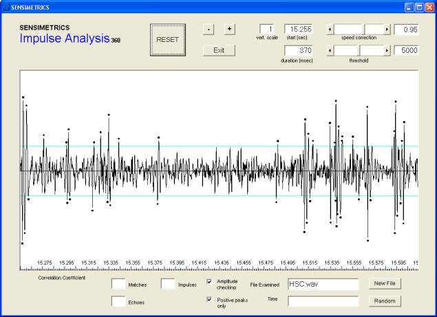
Figure 8 Initial appearance of the screen of the IMPULSES program before any analysis, after the sound recording file HSC.wav has been loaded. The screen shows 360 milliseconds of the recording, beginning just before the start (‘muzzle blast’) of the alleged grassy knoll gunshot at the left. The light horizontal lines show the threshold. Every impulse peak detected above the threshold is marked with a black dot by the program.
The program first finds all of the impulses displayed on the screen and marks each one with a black dot. Peaks below the center zero line are marked, too, because some of these are treated as echoes in the WA list. Next, the program counts the impulses that are within the time range and above the threshold, after these have been selected by the user. The program then finds the impulses that are within a millisecond of the echo times calculated by WA (see Figure 8). The program next computes the results of two different statistical tests to estimate the validity of the match between the WA list of echoes and the impulses in the part of the recording chosen for examination.
The scale used to determine the numerical value of the threshold is the dynamic range of digitized signal. All of the recordings used were normalized so that the level reached by the highest peak was 30935, which is 0.5 dB below the maximum level of 32768 obtainable for a 16-bit digital recording. The r.m.s. level of all three recordings was nearly identical for the 360-millisecond period; for the first 50 milliseconds after the muzzle blast impulse, the levels were –24.4 dB for the HSC recording; -17.7 dB for the FBI copy; and, -19.1 dB for the DPD copy.
One of the statistical tests is binary correlation (r), defined as the number of impulses that match predicted echoes, divided by the square root of all the impulses multiplied by all the echoes in the examined time period. The second test, the hypergeometric probability, is more complicated, but explanations can be found in textbooks on statistics. An especially clear explanation, with examples, can be found in: Douglas Downing and Jeffrey Clark, Statistics the Easy Way, Barron’s Educational Series, Inc. (1997), pp. 105-108.
By default, the IMPULSES program loads the file HSC.WAV, and displays 360 milliseconds containing ‘shot 3,’ as shown in Figure 8. Table 4 in WA (Figure 7 in this report) lists 26 echoes predicted to occur in this time period, the last at 369.1 milliseconds after the muzzle blast. As an example of the calculation of the correlation coefficient, suppose 15 impulses match the times of 15 of 17 predicted echoes exceeding the threshold. Assume further that there are 51 impulses higher than the threshold in the same time period. The binary correlation is 15 ÷ (square root of (51 x 17)), which is 0.5094. In the BBN report, 0.6 was set as the minimum correlation for an array of impulses to be accepted. The sequence in this example would therefore be rejected.
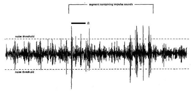
Figure 9 [a copy of Figure 2 from the WA report.] The dashed lines show the threshold to be exceeded for an impulse to be counted in the first of the correlation calculations described by WA. We have added the black bar at “a,” 50 milliseconds long, to show the period of the second calculation described by WA.
Here is a part of the WA report:
For the first calculation, the amplitude comparison level was set as in figure 2 [Figure 9 of this report]. Taking all of the factors discussed in section 5.4 into account, we found that 13 gunshot sounds (the muzzle blast and 12 of the predicted echoes) would have been loud enough to have been recorded at a level above the background noise. Eleven of these sounds coincided, within a ±1-millisecond window, with impulses that exceeded the amplitude comparison level. Including the leading impulse, which was identified as the muzzle blast, a total of 15 impulses exceeded this level.
The binary correlation coefficient was calculated as the number of gunshot sounds and impulses that coincided (11) divided by the square root of the product of the number of selected impulses (15) and the number of selected gunshot sounds (13). For these data, the binary correlation coefficient was calculated to be 0.79.
The test described here included the entire 360-millisecond segment, bracketed in Figure 9 with the legend, “segment containing impulse sounds.” We found the closest approximation to the position of the dashed line marked “noise threshold.” was a threshold of 5000.
Two prominent low-frequency tones were found in the spectrum of the recording, one at 56.5 Hz and the other at 59.5 Hz, where 60 Hz power line hum would be expected. These indicate speed errors of –5.8% and –0.8% respectively. If only the smaller error is corrected, on the assumption that this error was added by the machine used to make the copy, the larger error that remains is almost exactly –5%. This is the speed error that several investigators agree applies to the original recorder, and it is the value we applied. The program allows a large range of values to be used.
We read further that the 13 gunshot sounds found in the time period being analyzed included the gunshot (“muzzle blast”). Since this time was chosen by the investigators, it will necessarily be at the start of the series of sounds, and cannot be part of the correlation analysis. For this reason, the number of gunshot sounds must be reduced to 12. The same principle applies to the number of impulses that match gunshot sounds; the gunshot must not be counted, so this number must be reduced from 11 to 10. The total number of impulses during this period of the recording is also 14, not 15, if the gunshot is excluded. These changes do not cause the array to fall below the threshold correlation of 0.6, but they reduce the value of the correlation from 0.79 to 0.75.
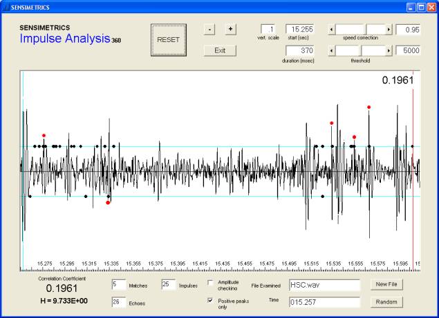
Figure 10.
The computer’s automatic analysis produced different results than those obtained by earlier investigators. We examined a 370-millisecond period, as this period contains all 26 of the predicted gun shot echoes. We matched the threshold shown in Figure 9 visually, as closely as we could, obtaining a threshold value of 5000 on the scale explained earlier. We also adjusted the speed compensation to .95 to correspond to the usual estimate of the speed error of the recording. We also removed amplitude checking, that is, the program ignored whether predicted echoes were above or below the threshold, so that all of the 26 predicted echoes were available for matching regardless of their amplitude.
Scanning the data (HSC.WAV) with the IMPULSES program, 25 impulses exceed the threshold. Of these 25 impulses, 5 are matches to predicted echoes, that is, within 1 millisecond of a predicted echo. These numbers result in a binary correlation of .196 (See Figure 10). Note that the vertical line indicating the end of the 370-millisecond period appears closer than expected to the muzzle blast, due to application of the speed correction value.
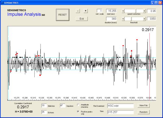
Figure 11.
After determining that the last of the predicted echoes (369.1 milliseconds) was not matched, we reduced the time span of the test to 360 milliseconds to exclude impulses in this region which might reduce the resulting correlation. We then gradually lowered the threshold to find the level at which 10 matches were found, as in the WA report. This occurred when the threshold was reduced to 3350 (see Figure 11). However, lowering the threshold also had the effect of increasing the total number of impulses detected, raising this number from 25 to 47, and producing a correlation coefficient of 0.2917, still below the desired value of 0.6.
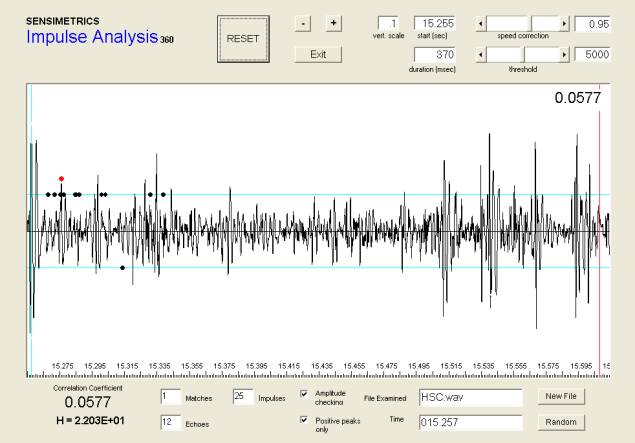
Figure 12.
The effect of amplitude checking was significant. Returning to the original threshold value of 5000 and adding amplitude checking, the computer program found only 1 match between impulses and predicted echoes (see Figure 12). In the array of predicted echoes, the corresponding threshold was estimated by finding the level that would be exceeded by the 12 largest predicted echoes, as measured on the diagram of the simulated grassy knoll shot in the WA report (the lower part of Figure 6 in this report). The resulting correlation coefficient is 0.0577.
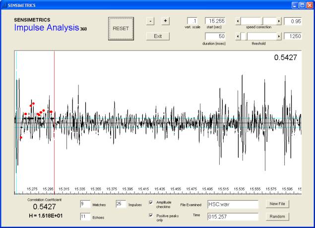
Figure 13.
WA describe a second correlation calculation using a specified time period of 50 milliseconds and a threshold set to one-fourth the value used in the first test.
For the second calculation … the delay time range over which impulses and echoes were compared was limited to the first 50 milliseconds … In this calculation, the amplitude comparison level was reduced to one-fourth of its value during the previous calculation, which placed it at a level just above that of very small peaks among the waveforms of the recorded impulses. Eighteen impulses exceeded this level. So would have the muzzle blast and all 11 echoes that were predicted to occur in the delay time range up to 50 milliseconds. Eleven of these sounds coincided, within ±1 millisecond, with one or another of the selected impulses. These data—11 coincident impulses and echoes, 12 gunshot sounds, and 18 impulses—resulted in a computed binary correlation coefficient of 0.75.
We analyzed the same time period in the same way, based on the method described by WA. Lowering the threshold to one-fourth the previous level (from 5000 to 1250) and leaving the other settings as in earlier tests, we obtained a correlation of 0.5427 for the 50-millisecond period, with 9 matches to the 11 echoes in this region, among 25 impulses (see Figure 13). Removal of amplitude checking had no effect on this result. Lowering the threshold lowered the correlation coefficient by increasing the total number of impulses admitted without increasing the number of matches.
The results obtained were dependent on the threshold selected and the value chosen for compensation of the speed error in the recording. One difference between the WA results and ours is in the total number of impulses counted. A larger number of these is detected and counted by the computer program than appears in the WA calculations.
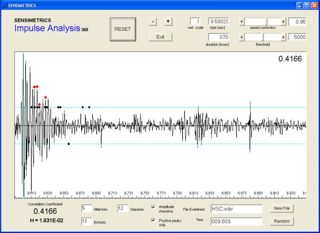
Figure 14. Correlation of the predicted echoes of ‘shot 3’ and a 370-millisecond segment of the HSC recording beginning about 6 seconds earlier than the muzzle blast attributed to ‘shot 3.’
We found that other noises in the recording were correlated to the predicted echo patterns nearly as well as the noise said to be the grassy knoll gunshot. For example, when we arbitrarily set the start of a “shot” at an impulse about 6 seconds earlier than the time of the impulse identified as the grassy knoll shot, the program gave a correlation of 0.4166 (see Figure 14).
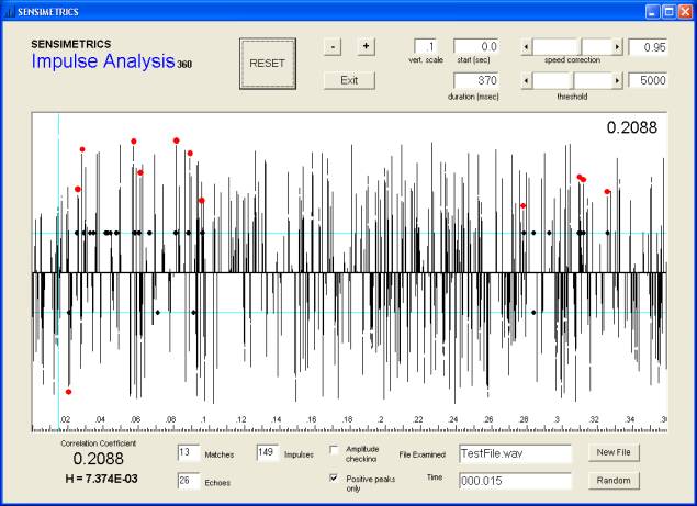
Figure 15 Correlation of the predicted echoes of ‘shot 3’ and a random array of impulses generated by the IMPULSES program.
We added a push-button to the IMPULSES program to generate random groups of impulses with approximately the same density as the impulses in the previously examined part of the recording and with random amplitudes (see Figure 15). When the arrays of random impulses were compared to the predicted gunshot echoes using the IMPULSES correlation routines, the numerical results were similar to those found for the alleged gunshots. The implication of this result is that if the statistical tests are accepted as determining that a group of impulses is gunfire from the grassy knoll, then random sounds generated by the computer appear as likely to be such gunfire as the suspected sounds in the Dictabelt recording.
We confirmed existing evidence that noises originally attributed to gunfire were recorded after the assassination.
One of the more difficult topics related to the recordings is the time when the sounds were recorded. There are several ways this might be determined. One way would be to measure the time with a stopwatch, counting from the most recent time announcement on the recording to the sounds thought to be gunshots. One difficulty with this method is that there could have been interruptions in the recording, making the recorded time less than the time that had actually passed. The recorder started only when a transmission was received; when no transmitter sent a message on its channel, a recorder switched itself off automatically.
The stopwatch method presents another problem. Time announcements made by the officer on duty were not made at exact intervals. The dispatcher usually looked at the clock and announced the time at the end of each message. However, this could happen in any part of the current minute. Often, no time was announced at the end of a transmission. At other times, several minutes might pass without an announcement.
The NAS panel was alerted by Steve Barber to an entirely different method for establishing the time of the alleged shots. Accompanying the popping noises and their ‘echoes,’ said to be the assassination gunshots, there is a voice message, faint but clearly audible. The sounds of the voice appear in figures in the BBN and WA reports. However, the origin and possible significance of the voice message were not identified or discussed in the BBN and WA reports. In the NAS report, it is shown that the voice message in the Channel 1 recording is essentially identical to a message sent on Channel 2 about a minute after the assassination. Clearly, if the popping and clicking sounds were recorded at the same time as the voice message, they could not possibly be sounds of the assassination gunfire, because the assassination had already taken place earlier.
This might have settled the matter by showing that the recorded sounds were simply irrelevant noises, no matter how closely the noises matched the predicted echoes. However, a theory was put forward that the noises were indeed the gunfire of the assassination, but that the voice message had somehow been added to the recording of the gunfire. Some argued that this may have been caused by accident; others implied that darker motives may have been at work. In fact, the idea that the voice and the impulses were recorded at different times is addressed in some detail in the NAS report, and there shown to be implausible.
We have taken a different approach to establishing the relation between the two sounds—the clicks and pops said to be gunfire and the voice—based on a well-known feature of many kinds of transmitting and recording equipment. The feature is usually called “AGC,” for “automatic gain control,” and it is cited in the WA report to explain why the amplitudes of the predicted echoes were not considered important.
Recording sounds at the correct level is often a problem, as anyone knows who has tried to make their own tape recording of music or speech. If the microphone is too close to a talker, for example, the sound level will be too high and recorded speech will be distorted. If the sound level is too low, on the other hand, background noise, such as static or tape hiss, will interfere with the quality of the recording. Most recorders have a level control that the user sets to make the recording loud and clear, but not so loud that it will be distorted. However, most people who use recorders for dictation or to record a meeting cannot stop to adjust the recording level for each talker. For this reason, many recorders have “automatic gain control,” or “AGC,” to estimate and set a good recording level automatically.
AGC can have interesting effects during certain kinds of recordings. If a recording consists of speech interrupted by gunshots, for example, the AGC will respond to the loud gunshots by reducing the recording level automatically, usually in a fraction of a second. For a short time, the level will be too low to make a good speech recording. After a fraction of a second, because speech is the only sound being recorded, the AGC will recover and restore the level to its earlier setting. This effect is of interest in the case of the Dallas recording.
If the speech and the gunshots are being recorded at the same time, every gunshot will cause the recording level to decrease for a short time. If the speech and gunshots were not recorded at the same time, the shots will have no effect on the speech level. Or if the ‘gunshots’ are scratches made on the Dictabelt after recording, the scratches will have no effect on the recorded speech level.
In their report to the congressional select committee, investigators cited the automatic gain control (AGC) feature in the police radio apparatus as an explanation for the difference between the level of the impulses on the police tape recording and the levels in the 1978 gunshot test recordings. The explanation in the WA report reads:
The DPD radio dispatching system contained a circuit that would have greatly affected the relative strengths of the recorded echoes of a muzzle blast. This circuit, the automatic gain control (AGC), limited the range of variations in the levels of signals by reducing the levels of received signals when they were too strong and increasing their levels when they were too weak. It responded very rapidly to a sudden increase in the level of a signal, but comparatively slowly to a sudden reduction in a signal level. Consequently, the response of the AGC to the sound of a muzzle blast would greatly reduce the recorded levels of echoes and background noise received shortly afterward. Progressively during the next 100 milliseconds, the AGC would allow the recorded levels of received signals to increase until full amplification was finally restored. The effect on the predicted echoes would be to make the recorded levels of late-arriving echoes very nearly the same as those of the early ones. Concurrently, the recorded background noise would gradually rise to its level before the muzzle blast was received.
At the beginning of the BBN report is a list of questions and answers. One of these is:
5. Did the range of amplitude (loudness) of the impulse patterns resemble that of the echo patterns produced by the test shots?
Yes. Processing the echo patterns of the test shots through a radio receiver like that used in the DPD recording system showed similar compression of the range of amplitude of recorded signals with respect to the range of the signals fed into the receiver.
The compression described could have been the result of overload of the circuits by an extremely loud sound. Even a cursory visual inspection of the ‘gunfire’ waveforms, especially the waveform of ‘shot 3,’ shows a pattern of impulse magnitudes that is very unusual when compared to other instances of a loud sound followed by echoes. This is especially noticeable in the Figure 6. There, a test shot fired from the grassy knoll and its echoes, are compared to the part of the DPD recording said to contain ‘shot 3.’ Although the effects of AGC on impulse height may have caused the magnitudes of the earliest impulses to decrease or fluctuate, the considerable height of the later impulses is the opposite of what would be expected of the last echoes in such a series. These impulses have no visible counterparts in the test gunshot (See Figure 6)
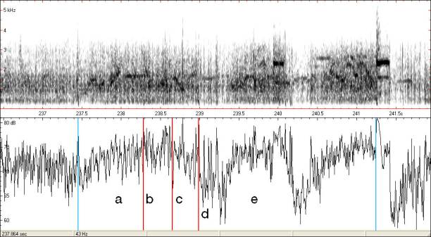
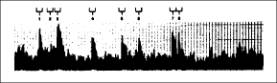
Figure 16. (Upper part of figure) Spectrogram of a portion of the DPD Channel 1 recording containing ‘shot 3,’ ‘shot 4,’ and about 4 seconds of additional time. The blue lines (237.45 and 241.25 seconds) mark the start and end of a recorded speech transmission originating on Channel 2 and appearing on Channel 1. (Lower part of figure) Plot of the energy in the recorded signal in dB (scale at left). a = noise and speech before gunshot; b = ‘shot 3’; c = final echoes of ‘shot 3’; d = ‘shot 4’; e = noise and speech after ‘gunshot’ echoes. The generally downward trend after b and c indicates the action of the AGC circuit in response to the loud noise of ‘shot 3’ and its echoes. Sounds that do not produce such a trend are probably noises caused by scratches or debris in the Dictabelt.
In the spectrogram that forms the upper part of Figure 16, at 237.45 seconds, a very strong impulsive sound is shown as a vertical line. This is followed by indications of a distorted speech transmission, the black, smudge-like diagonal and horizontal lines. In the lower part of the figure, where the signal energy is plotted, at the letter a, the level of the initial speech signal and background noise average about 72 dB on the scale at the left. At the letter b, ‘shot 3’ is fired, and the average level starts to descend immediately. Just before c, a burst of very loud sounds again causes the average level to drop, a trend that continues until d, when ‘shot 4’ occurs, forcing the average level to fall even lower.
More loud noise impulses follow, but instead of falling, the level continues to climb. This indicates that these noises are not part of the original recording, but are scratches or other damage to the Dictabelt acquired after recording. The fluctuating level of the speech and noise, seen in the energy plot, then rises in the region e to the level it initially had at a, until a loud tone at about 2400 Hz (at 240 seconds) triggers the AGC again and the level drops steeply.
Most, but not all of the recorded noises said to be gunfire caused the AGC to reduce the sound level of the speech and background noise in the recording. This could only have happened if the gunshot-like sounds were recorded at the same time as the voice message. Otherwise, there would have been no reason for the speech and noise to drop in level at exactly those times.
There is no ambiguity regarding the content of the voice transmission. In the NAS review, spectrograms and other detailed analytic results are cited to show that the voice message is one that was transmitted on Channel 2 about a minute after the assassination. The effect of AGC action on the level of other sounds is also discussed in the NAS review. However, the interaction of the AGC, the impulses and the speech indicate that most of the gunshot-like sounds were recorded during the voice transmission, that is, after the assassination. Others, equally loud or even louder, had no effect on the AGC and are probably scratches or dirt on the recording surface.
In light of this data, it becomes even more difficult to support the idea that the impulses are the sounds of the assassination. The data indicate that the speech was not superimposed on the noise because of a mistake or an attempt at deception—they are together because they were recorded at the same time.
Three different copies of the Channel 1 recording were available to us in our work. The recordings are compared in Figure 17, which illustrates the differences in waveforms of the same events in each of the three recordings—the event identified as the third gunshot. The results of applying statistical tests to verify this identification vary considerably.
“HSC” shows part of the waveform from a copy of the recording used by BBN and WA and subsequently examined by the NAS committee. We digitized the waveform from the analog tape and concluded, after comparing our computer screen displays to the illustrations in the BBN and WA reports, that the NAS copy was essentially identical to the recording depicted by BBN and WA, showing the effects of the digital filtering they had applied to the DPD original.
“DPD” is from a copy of the recording made by James Bowles of the Dallas Police Department.
“FBI” is from the copy of the Channel 1 recording made by the F.B.I. during the NAS review. This copy exhibits significant defects not present in the other two recordings.
The distinctive appearance and sound of the HSC recording can be attributed at least in part to the digital filtering applied to the recording before analysis.
The recorded outputs from both filters for the full 5 minutes were compared, examined, and plotted on a scale where 5 in. equals 1/10 sec. …
One filter was an adaptive filter, whose function is described in the BBN report.
One property of periodic components is that, given sufficient past history, they can be predicted; indeed, a perfectly periodic signal can be predicted perfectly. The filter “learns” from the past history of the signal, estimates the signal for the next time period, and subtracts its estimate from the input. What is left are those portions of the signal that the filter cannot estimate, i.e., the random components.
We examined and tested all three versions of the same event (“shot 3”) using the IMPULSES program. For all three recordings, we set the analysis time to 370 milliseconds, adjusted the level threshold to give the highest value of correlation, and held the speed correction at 0.95, corresponding to a recording speed error of -5%. We obtained the following results for the values of binary correlation (r):
HSC 0.1961 threshold = 5000
FBI 0.2993 threshold = 7400
DPD 0.3849 threshold = 6950
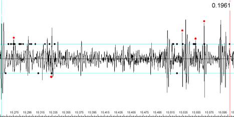
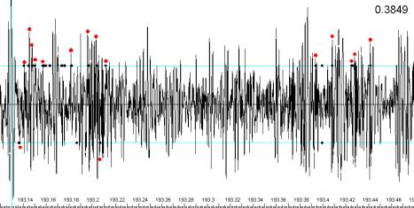
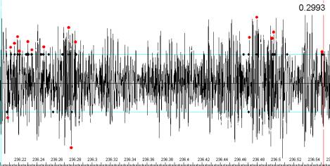
Figure 17. 360-millisecond segments of three versions of the Dallas Police Department Dictabelt recording. From top, HSC (the version provided to the NAS for their study), FBI (made in the course of the NAS study) and DPD (made by James C. Bowles, Head of the of the Dallas Police Communication Department in 1963).
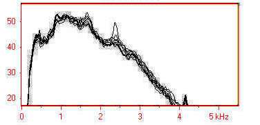
Figure 18. Superimposed images of spectra of three-second segments of noise in the Channel 1 recording. The samples were taken at the following times (in seconds): 70, 142, 156, 171, 183, 214, 256, and 298. One spectrum contained a brief tone producing the peak at 2.4 kHz for a fraction of a second.
For several of the five minutes, the recording consists of little more than loud noise. The noise was examined by BBN and compared to a recording of a motorcycle they had made. Features that would allow the noise to be identified as a motorcycle could not be found. Here is a description of this work in the BBN report.
Our interpretation of the sounds on the Channel 1 tape would have been made much easier if we had had some knowledge of the movements of the motorcycle carrying the microphone. For example, if we had had information on when the motorcycle was moving steadily (along a straight street), slowing down and possibly shifting gears to turn a corner, or stopping, we might have been able to infer whether these movements were consistent with travel into or through Dealey Plaza . However, we did not have this information. … [An] autocorrelation analysis program was applied to the stuck transmission period on the Channel 1 tape. The results showed no periodicity that we could attribute to motorcycle engine firing. As a test case, this program was also applied to a high-fidelity recording of motorcycle engine noise, and it clearly showed the known periodicity of the test signal. Although our failure to detect the motorcycle engine periodicity is puzzling, it is consistent with our inability to perceive the engine firing clearly when we are listening to the tape, and it is also somewhat consistent with the failure of the adaptive noise-canceling filter to filter out a coherent motorcycle engine sound signal.
We analyzed the noise and found that its spectral characteristics hardly changed at all over the five-minute period. This is true of segments taken as samples in quite different places in the recording, both before and after the sounds said to be assassination gunfire (see Figure 18).
One possibility is that the transmitter microphone, that is, the motorcycle did not move during the five-minute period, but was parked at a location where there was a high noise level. Other sounds might have been recorded briefly when other transmitters, producing a stronger signal than the stuck transmitter at the police headquarters receiver, ‘captured’ Channel 1.
5. A Critical Occurrence of Crosstalk?
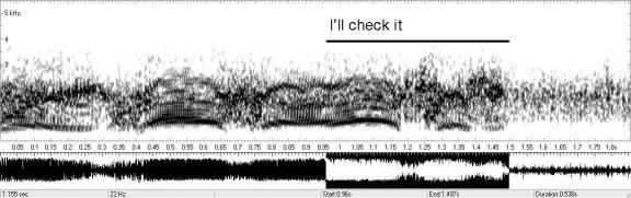
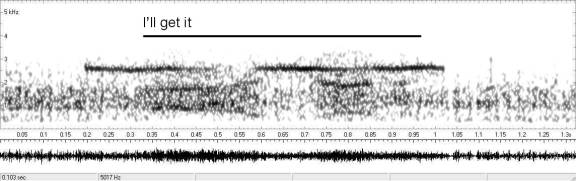
Figure 19. Spectrograms of voice messages from Channel 2 (above) and from Channel 1 (below). The suggestion has been made that the two messages were identical and could be used as a timing reference. The time scale in the upper spectrogram is 2 seconds, in the lower, 1.33 seconds. Both utterances have approximately the same duration.
Since the two formal investigations (BBN and NAS) have been published, arguments for a different method of time calibration of the recording have been presented, based on the occurrence of voice messages on Channel 1 and Channel 2 said to be identical. The proposals appear to have been motivated by the discovery of the crosstalk message transmitted after the assassination, which is heard in the background during the sounds said by BBN and WA to be the gunfire of the assassination.
It has been proposed that the alternate message might be used as a time reference, placing the time of the gunshot sounds at the time of the assassination and vindicating the claim that a shot had been fired from the grassy knoll.
It is not difficult to show by spectrographic analysis that the two recordings cited contain two entirely different messages. On the Channel 1 recording, the words are, “I’ll get it.” On Channel 2, a longer message concludes, “I’ll check it.” The acoustic content of the two transmissions can be seen to be very different (see Figure 19).
The messages are not the same, and so are not useful for timing purposes.
Following (Figure 20) are plots of the four gunshots identified in the DPD recordings by BBN, and listed in their report to the congressional subcommittee. We have located and plotted the beginning of each shot using the BBN timing.
The BBN report states:
Examination of the entire 5-minute segment did not reveal sufficiently similar impulse patterns elsewhere on the tape to discount gunfire as the source of these four patterns.
The following also appears in the report:
These plots revealed five impulse patterns introduced by a source other than the motorcycle. Upon closer examination, all but one of these patterns were sufficiently similar to have had the same source, and the impulses contained in these patterns appeared to have shapes similar to the expected characteristics of a shock wave and of a muzzle blast. The remaining pattern was sufficiently different in amplitude and duration as to have been caused by a different source .
Oswald allegedly fired shots 1, 2 and 4 with one rifle from a window of a building overlooking Dealey Plaza. However, no visible details of the recording waveforms suggest that they came from the same source, or provide a means of differentiating them from other impulsive sounds in the same part of the recording. There would be a closer resemblance between 1 and 2 if the starting time of 1, as shown here and in the figure in the BBN report, was shifted from (a) to a time about 0.25 second later (b), as it is in the text of the report.
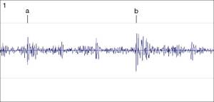
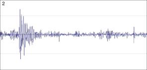
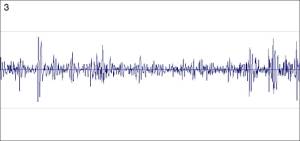
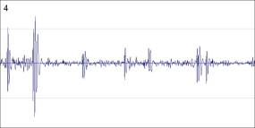
Figure 20. The four gunshot waveforms in the DPD recording after filtering applied by BBN. The time scale in each picture is the same. Gunshot 1 is described in the text of the BBN report as starting with the muzzle blast at b, while the illustration in the report shows the shot starting at a.
Summary
Studies of a 1963 Dallas Police radio recording identified four groups of impulses as sounds of the gunfire of the assassination of President John F. Kennedy. Three of the gunshots were reported to be those allegedly fired by Lee Harvey Oswald. A fourth gunshot was reported to have originated from behind a fence on the “grassy knoll,” indicating the presence of a second assassin.
A new analysis of the recording, with various steps carried out automatically, has produced different results. Among these are statistical results indicating that the gunfire noises are not unusually different from other noises in the recording; spectral data on background noise demonstrating that the noise is not the kind expected from motorcycles or other types of moving vehicles; and, analysis of fluctuations of level in the recording indicating, as earlier work has already shown, that the noises said to be assassination gunfire were recorded during a voice transmission that was made after the assassination.
The suggestion that the timing of another voice message was transmitted on another channel, and could establish that the examined noises had been recorded during the assassination, was found to be mistaken.
This study was commissioned by Medstar Television and Court TV.
Michael Joseloff, producer of the television program which reports much of this work, made important contributions to the form and content of the report. He was exceptionally understanding and encouraging.
I wish also to express my gratitude to my colleagues at Sensimetrics Corporation, especially Pat Zurek, Kenneth Stevens, Oded Ghitza, Robert Beaudoin and Tom von Wiegand, who listened patiently to my periodic accounts of the details and progress of the work.
The copies of the 1963 recordings used for analysis were digitized by Mark Donahue at Soundmirror, Inc., of Jamaica Plain, Massachusetts.
[BBN] Barger, James E., Scott P. Robinson, Edward C. Schmidt, and Jared J. Wolf (1979), Analysis of Recorded Sounds Relating to the Assassination of President John F. Kennedy. Prepared for Select Committee on Assassinations. http://history-matters.com/archive/jfk/hsca/reportvols/vol8/pdf/HSCA_Vol8_AS_2_BBN.pdf
[WA] Weiss, Mark R. and Ernest Aschkenasy (1979), An Analysis of Recorded Sounds Relating to the Assassination of President John F. Kennedy. Prepared for Select Committee on Assassinations, U.S. House of Representatives. http://history-matters.com/archive/jfk/hsca/reportvols/vol8/html/HSCA_Vol8_0004a.htm
[NAS] Report of the Committee on Ballistic Acoustics (1982). Commission on Physical Sciences, Mathematics, and Applications. Washington, D.C., National Academies Press. http://www.nap.edu/execsumm/NI000372.html
112403